

Hardware Efficient Randomized SVD

TL;DR
Replacing FP32 Householder QR with 16-bit matrix multiplications and Cholesky QR in randomized SVD achieves a 4.1× speedup over torch.svd_lowrank for online KV-Cache compression, with negligible accuracy loss on the RULER benchmark.
1. Introduction
Large Language Models are increasingly deployed at long context lengths — hundreds of thousands of tokens — creating a severe memory bottleneck. During autoregressive generation, the attention mechanism caches every previously computed Key and Value (KV) state. This KV-Cache grows as $\mathcal{O}(L \cdot d \cdot N_\text{layers})$, where $L$ is the sequence length and $d$ the per-head hidden dimension. For a 32-layer model with head dimension 512 at 128k-token context in 16-bit precision, the KV-Cache alone requires tens of gigabytes — often comparable to the model weights themselves.
SVD-based compression addresses this directly. Recent work, xKV [5], observes that the dominant singular vectors of KV-Caches are well-aligned across adjacent layers. Concatenating the KV-Caches of $G$ adjacent layers and applying one shared SVD extracts a basis common to all of them — achieving up to 8× higher compression while maintaining accuracy. However, that memory saving comes at a cost: xKV must compute SVD online during the prefill phase of every request, and this step becomes a significant and growing fraction of prefill latency.
In this blog post we will walk through:
- How SVD compresses matrices in general.
- How xKV applies SVD to the KV-Cache.
- Why existing PyTorch SVD implementations — both full and randomized — remain a bottleneck online.
Then we present two targeted optimizations to randomized SVD — 16-bit matrix multiplications for the power iteration (unlocking Tensor Cores) and a numerically robust Cholesky QR for orthogonalization — that together deliver a 4.1× speedup over torch.svd_lowrank with negligible accuracy loss on RULER.
Our implementation is publicly available at github.com/bairixie/kv-svd, evaluated within the xKV framework on an NVIDIA RTX A6000.
2. Background
2.1 Singular Value Decomposition
For any real matrix $X \in \mathbb{R}^{m \times n}$, the Singular Value Decomposition (SVD) is [7]:
\[X = U \Sigma V^\top\]where $U \in \mathbb{R}^{m \times m}$ and $V \in \mathbb{R}^{n \times n}$ are orthogonal matrices, and $\Sigma \in \mathbb{R}^{m \times n}$ is diagonal with non-negative entries $\sigma_1 \geq \sigma_2 \geq \cdots \geq \sigma_r \geq 0$, $r = \min(m, n)$.
Truncating to the top-$k$ components gives the rank-$k$ approximation $X_k = U_k \Sigma_k V_k^\top$. The Eckart-Young theorem guarantees it is optimal:
\[\|X - X_k\|_F = \min_{\text{rank}(Y) \leq k} \|X - Y\|_F = \sqrt{\sigma_{k+1}^2 + \sigma_{k+2}^2 + \cdots}\]No other rank-$k$ matrix achieves smaller error — this is the theoretical foundation for SVD-based compression throughout machine learning.
2.2 SVD for Matrix Compression
Taking the three truncated matrices ($U_k, \Sigma_k, V_k^\top$) after applying SVD, we can absorb the $\Sigma_k$ into either $U_k$ or $V_k^\top$ to derive:
- $A = U_k \Sigma_k \in \mathbb{R}^{m\times k}$
- $B = V_k^\top \in \mathbb{R}^{k\times n}$
We term $A$ as the basis, and $B$ as the reconstruction matrix. Looking carefully at the shape of the matrices, performing a rank-$k$ SVD on a matrix $X$ can yield a compressed representation of space complexity $\mathcal{O}(mk+nk)$. When $k$ is sufficiently small, we successfully yield a more compact representation for the original matrix $X$ using a pair of smaller matrices.
3. SVD for KV-Cache Compression
3.1 Review of xKV
Now that we understand how SVD can compress generic tensors, we turn to how it applies to the KV-Cache, which can itself be viewed as a matrix.
Concretely, at prefill we have per-layer KV-Caches $X_\ell \in \mathbb{R}^{L \times d}$, with sequence length $L$ and per-head dimension $d$. Rather than treat each layer in isolation, we concatenate the caches of $G$ adjacent layers into a single tall matrix
\[\mathbf{X} \;=\; \bigl[X_{\ell_1}, \ldots, X_{\ell_G}\bigr] \;\in\; \mathbb{R}^{L \times (Gd)}.\]Following the basis/reconstruction decomposition from Section 2.2, a rank-$k$ SVD of $\mathbf{X}$ — with the reconstruction matrix split column-wise by layer — yields a shared basis $A$ alongside $G$ layer-specific reconstruction slices $B_{\ell_i}$:
\[\mathbf{X} \;\approx\; A\,\bigl[B_{\ell_1}, \ldots, B_{\ell_G}\bigr], \qquad A \in \mathbb{R}^{L \times k},\;\; B_{\ell_i} \in \mathbb{R}^{k \times d}.\]Each layer’s cache is recovered by $X_{\ell_i} \approx A\,B_{\ell_i}$, so one SVD compresses all $G$ layers jointly with total storage $\mathcal{O}(Lk + Gdk)$ in place of $\mathcal{O}(GLd)$. The per-layer baseline is simply $G = 1$; there is no fundamental split between “single-layer” and “cross-layer” SVD, only a choice of $G$.
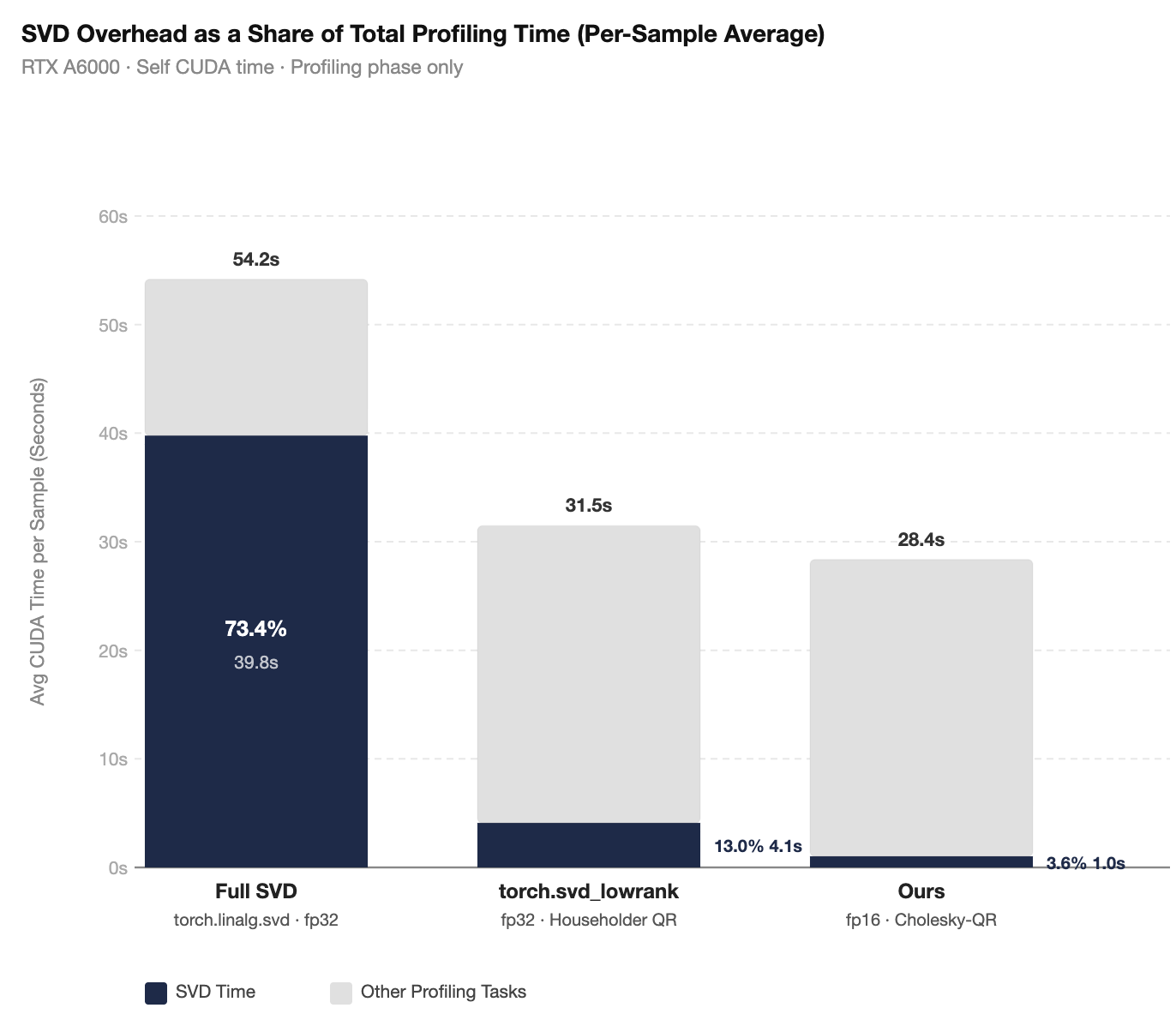
In xKV, SVD is performed online after prefill to better capture the changing dynamics of the inputs for accuracy preservation. While applying SVD to the KV-Cache effectively reduces its size, it is not a free lunch: on an RTX A6000, PyTorch’s torch.linalg.svd (full SVD) alone accounts for 73.4% of per-sample profiling time — not viable for production.
4. Toward Efficient SVD Computation — Randomized SVD
4.1 Compute Only the Needed Singular Vectors
For KV-Cache compression we only need the top-$k$ singular vectors. Full SVD computes all $\min(m, n)$ components — often $10\times$ to $100\times$ more than necessary. One direct intuition for optimizing SVD is therefore to compute only the singular vectors we actually need, which is exactly what Randomized SVD does.
Randomized SVD [1] reduces the dominant cost from $\mathcal{O}(mn^2)$ to $\mathcal{O}(mnk)$ by identifying the $k$-dimensional dominant subspace directly. We benchmark PyTorch’s off-the-shelf torch.svd_lowrank and observe SVD’s share of per-sample profiling time drop from 73.4% to 13.0%.
4.2 Algorithm Behind Randomized SVD
The algorithm proceeds in four stages.
Stage 1 — Setup. Transpose if $m < n$ so all stages operate on a tall matrix. Resolve working dtype; allocate $\mathbf{I}_{k+p}$.
if m < n:  A, M = A.T, M.T
X    = cast(A, working_dtype)
eye_q = identity(k + p, dtype=working_dtype)
Stage 2 — Random Projection. Draw $R \in \mathbb{R}^{n \times (k+p)}$ and form sketch $Y = (A - M)R$. Orthonormalize to initial basis $Q$.
R = randn(n, k + p, dtype=working_dtype)
Y = (A - M) @ R
Q = orthonormalize(Y)
Stage 3 — Power Iteration. Alternate $A^\top$ and $A$ to sharpen $Q$:
for _ in range(n_iter):
    Q = orthonormalize((A - M).T @ Q)
    Q = orthonormalize((A - M)  @ Q)
Each iteration amplifies eigenvalue ratios by $(\sigma_i / \sigma_j)^{2n_\text{iter}}$, rapidly concentrating $Q$ on the dominant subspace. With $n_\text{iter} = 4$, this stage accounts for 62–80% of total SVD time depending on implementation.
Stage 4 — Project and Recover.
B       = Q.T @ (A - M)                    # shape: (k+p) × n
U_, S, Vt = svd(B.float(), full=False)     # FP32: torch.linalg.svd rejects 16-bit input
U       = Q @ U_
# truncate to top-k; undo transpose if needed
Total cost is dominated by the $(2n_\text{iter} + 1)$ multiplications with $A$, each $\mathcal{O}(mn(k+p))$ — a factor of $n/(k+p)$ cheaper than full SVD.
4.3 Limitations of the Existing Implementation (torch.svd_lowrank)
1. FP32 throughout — no Tensor Core utilization. All matrix multiplications in Stages 1–3 run in FP32. Modern NVIDIA GPUs (Ampere, Hopper) deliver substantially higher throughput for 16-bit operations via Tensor Cores. In our profiling, the matrix-multiply sub-cost of the power iteration alone is 91.5 s.
2. Householder QR is the orthogonalization bottleneck. Each orthonormalize(·) call invokes torch.linalg.qr. While backward-stable, Householder QR’s sequential panel factorizations expose limited parallelism for tall-and-skinny shapes ($m \gg k+p$). The QR sub-cost in the power iteration is 222.6 s — 56.9% of the total 392.0 s wall-clock time in randomized SVD.
5. Hardware-Efficient Randomized SVD (Our Method)
5.1 Overview
Our method is structurally identical to torch.svd_lowrank. We introduce exactly two modifications: (1) 16-bit computation for all large matrix operations, and (2) Cholesky QR for orthogonalization. The design principle is to maximize 16-bit coverage for bandwidth-bound operations while performing a surgical FP32 upgrade only where precision is non-negotiable.
| Stage | Operation | torch.svd_lowrank |
Ours (16-bit path) |
|---|---|---|---|
| 1. Setup | Cast input, $\mathbf{I}_{k+p}$ | FP32 | 16-bit |
| 2. Random Projection | $Y = AR$, orthogonalize | FP32 · Householder QR | 16-bit matmul · Cholesky QR |
| 3. Power Iteration | $A^\top Q$, $AQ$, orth. | FP32 · Householder QR | 16-bit matmuls · Cholesky QR |
| 4a. Projection | $B = Q^\top(A{-}M)$ | FP32 | 16-bit |
| 4b. Small SVD | $\text{svd}(B)$ | FP32 | FP32 (PyTorch constraint) |
| 4c. Lift & truncate | $U = Q\hat{U}$ | FP32 | 16-bit |
Two design choices deserve emphasis. chol_qr is 16-bit-in / 16-bit-out with an internal FP32 upgrade: it receives a 16-bit matrix, immediately upcasts to FP32 for Gram matrix computation and Cholesky factorization (where numerical stability matters), then returns $Q$ in 16-bit. Inter-stage memory traffic stays in 16-bit; the factorization runs in FP32.
Stage 4b must remain FP32 because torch.linalg.svd raises a runtime error on 16-bit input — a hard PyTorch constraint, not a precision choice. Fortunately $B$ has shape $(k+p) \times n$ (e.g., $4 \times 512$ with $p = 0$), making this cost negligible.
5.2 Optimization 1: 16-bit Power Iteration
The power iteration consists of repeated large matrix multiplications:
\[Q \;\leftarrow\; \text{orth}(A^\top Q), \qquad Q \;\leftarrow\; \text{orth}(A\,Q)\]where $A \in \mathbb{R}^{L \times (Gd)}$ is the grouped KV-Cache. Three properties make this ideal for precision reduction:
-
Memory-bandwidth bound. The dominant cost is reading $A$ from GPU HBM. Reducing element size from 32-bit to 16-bit directly halves memory traffic.
-
Approximation-tolerant. The power iteration estimates a subspace, not an exact result. 16-bit rounding errors are equivalent to a small perturbation of the input — precisely the regime that randomized SVD handles robustly [1]. Subsequent iterations further suppress single-step errors.
-
Not the final computation. Stage 3 produces only an intermediate orthonormal basis $Q$. Singular values are computed in Stage 4b in FP32.
On RTX A6000, switching from FP32 to 16-bit reduces the matrix-multiply sub-cost from 91.5 s → 22.5 s (4.1×), consistent with expected gains from Tensor Core utilization and halved memory bandwidth. Our implementation supports both IEEE float16 and bfloat16; both yield essentially identical task accuracy and performance on these workloads.
5.3 Optimization 2: Numerically Robust Cholesky QR
Each orthonormalize(Y) call takes $Y \in \mathbb{R}^{m \times (k+p)}$ with $m \gg k+p$. All internal computation is FP32; the result is cast back to 16-bit on return.
Basic Cholesky QR
Cholesky QR [2] exploits the algebraic identity: if $Y = QR$ then $Y^\top Y = R^\top R$. In other words, the $R$ factor we want is simultaneously the Cholesky factor of the small Gram matrix $G = Y^\top Y$. This turns orthogonalization into three BLAS calls: one SYRK to form $G$, one Cholesky on the tiny $(k+p)\times(k+p)$ matrix, and one triangular solve (TRSM) to recover $Q = Y R^{-1}$.
Compared to Householder QR, Cholesky QR requires roughly half the total flop count for tall-skinny matrices [2]. SYRK and TRSM are Level-3 BLAS routines achieving near-peak GPU throughput; Householder QR’s sequential panel updates expose far less parallelism for small $k+p$.
Gram Matrix Symmetrization
Before factorizing, we explicitly symmetrize $G$:
\[G \;\leftarrow\; 0.5\,(G + G^\top)\]Floating-point rounding in $Y^\top Y$ accumulates small off-diagonal asymmetries. Explicit symmetrization eliminates this drift before it reaches cholesky_ex, reducing spurious factorization failures.
Adaptive Shift Regularization
Following the shifted Cholesky QR framework of Fukaya et al. [3], we add a scale-invariant diagonal regularization:
\[G_\text{shifted} = G + \varepsilon \cdot \text{scale} \cdot I, \quad \text{scale} = \text{mean}(\text{diag}(G)).\text{clamp}(\min=10^{-12})\]We drive this with torch.linalg.cholesky_ex, which returns an info tensor rather than raising an exception — making batch-aware failure detection easy. Starting from $\varepsilon_0 = 10^{-5}$, we try the shifted Cholesky; on any batch element’s failure we multiply $\varepsilon$ by 10 (capped at max_eps) and retry, up to max_tries attempts. In the common case — a well-conditioned $Y$ — the first attempt succeeds and the shift is numerically negligible; the exponential backoff only kicks in for progressively more ill-conditioned inputs, with no manual tuning required.
Eigh SPD-Repair Fallback
If all shifted Cholesky attempts fail, we don’t give up — instead we reconstruct a strictly positive definite approximation of $G$ and Cholesky-factorize that [4]. Concretely: eigendecompose $G = V\Lambda V^\top$, clamp the eigenvalues to be at least $\max(10^{-4}, \varepsilon)$, reassemble $G_\text{spd} = V\bar{\Lambda} V^\top$, and Cholesky-factor that instead.
This reconstruct-then-Cholesky design keeps the downstream triangular solve well-conditioned: $R$’s diagonal entries are bounded away from zero by construction, so we never amplify the clamped eigenvalue errors.
Householder QR as Final Safety Net
If even the eigh path raises an exception, we fall back to standard Householder QR via torch.linalg.qr(Y, mode="reduced"). This recovers exactly the behavior of torch.svd_lowrank, making our implementation strictly more robust than the baseline — it can never perform worse. In practice, this path is almost never triggered; it exists purely as a correctness guarantee.
Putting It All Together
Putting the four pieces into one routine gives the complete chol_qr we use in Stages 2 and 3. It’s 16-bit-in / 16-bit-out, with the internal factorization lifted to FP32 for stability:
@torch.no_grad()
def chol_qr(
    Y_fp16: Tensor,
    eye: Tensor,
    base_eps: float = 1e-5,
    max_eps: float = 10.0,
    max_tries: int = 6,
    use_eigh_last: bool = True,
) -> Tensor:
    # Work in float32 internally for numerical stability.
    Y = Y_fp16.float()

    # Gram matrix G = Y^H Y, symmetrized to remove finite-precision drift.
    G = torch.matmul(Y.mH, Y)
    G = 0.5 * (G + G.mH)

    # Scale-invariant jitter derived from the mean of the diagonal.
    d = torch.diagonal(G, dim1=-2, dim2=-1)
    scale = d.mean(dim=-1, keepdim=True).clamp_min_(1e-12).unsqueeze(-1)

    # Shifted Cholesky with exponential backoff on eps.
    eps = base_eps
    for _ in range(max_tries):
        R, info = torch.linalg.cholesky_ex(G + (eps * scale) * eye, upper=True)
        if (info == 0).all():
            Q = torch.linalg.solve_triangular(R, Y, upper=True, left=False)
            return Q.to(Y_fp16.dtype)
        eps = min(eps * 10.0, max_eps)

    # Fallback 1: eigh-based SPD repair, then Cholesky on the repaired matrix.
    if use_eigh_last:
        try:
            L, V = torch.linalg.eigh(G)
            L = torch.clamp(L, min=max(1e-4, eps))
            G_spd = torch.matmul(V, torch.matmul(torch.diag_embed(L), V.mH))
            R = torch.linalg.cholesky(G_spd, upper=True)
            Q = torch.linalg.solve_triangular(R, Y, upper=True, left=False)
            return Q.to(Y_fp16.dtype)
        except Exception:
            pass

    # Fallback 2: plain Householder QR — matches torch.svd_lowrank exactly.
    Q, _ = torch.linalg.qr(Y, mode="reduced")
    return Q.to(Y_fp16.dtype)
The structure mirrors the progression in this section: the fast happy path (shifted Cholesky) handles the overwhelming majority of inputs, and each fallback layer exists to absorb a progressively rarer failure mode without ever being slower than the baseline.
6. Experiments
6.1 Setup
Hardware. Single NVIDIA RTX A6000 GPU. All timing figures report self CUDA time via the PyTorch profiler, collected during the profiling (prefill) phase only — steady-state decode-phase evaluation is left for future work.
Benchmark. We evaluate within the xKV framework [5] at github.com/abdelfattah-lab/xKV. Accuracy is measured on four RULER subtasks [6]: Frequent Word Extraction (FWE), NIAH MultiKey, NIAH Single1, and Variable Tracking (VT). RULER is a long-context evaluation suite designed to stress KV-Cache compression artifacts by requiring retrieval and reasoning at various positions within a long context.
Configuration. Layer group size $G = 4$, $n_\text{iter} = 4$ power iteration steps, oversampling $p = 4$. Full SVD was profiled at approximately 10 samples due to OOM at 96 samples; other methods ran for 96 samples.
Methods compared:
torch.linalg.svd— full SVD, FP32 (memory-limited reference only)torch.svd_lowrank— randomized SVD, FP32, Householder QR- Ours — fp16 · Cholesky-QR (this work)
6.2 End-to-End SVD Latency
Takeaways.
- Full SVD is not viable: it consumes 73.4% of profiling time per sample and causes OOM at 96 samples.
torch.svd_lowrankis still a bottleneck: 13.0% SVD overhead (4.1 s/sample) limits throughput.- Ours drops SVD to 3.6%: per-sample SVD time falls from 4.1 s → 1.0 s (4.1×), a level where SVD is no longer a dominant cost.
| Method | Total / sample | SVD / sample | SVD % |
|---|---|---|---|
Full SVD (torch.linalg.svd, fp32) |
54.2 s | 39.8 s | 73.4% |
torch.svd_lowrank (fp32 · Householder QR) |
31.5 s | 4.1 s | 13.0% |
| Ours (fp16 · Cholesky-QR) | 28.4 s | 1.0 s | 3.6% |
6.3 Stage-Level Breakdown
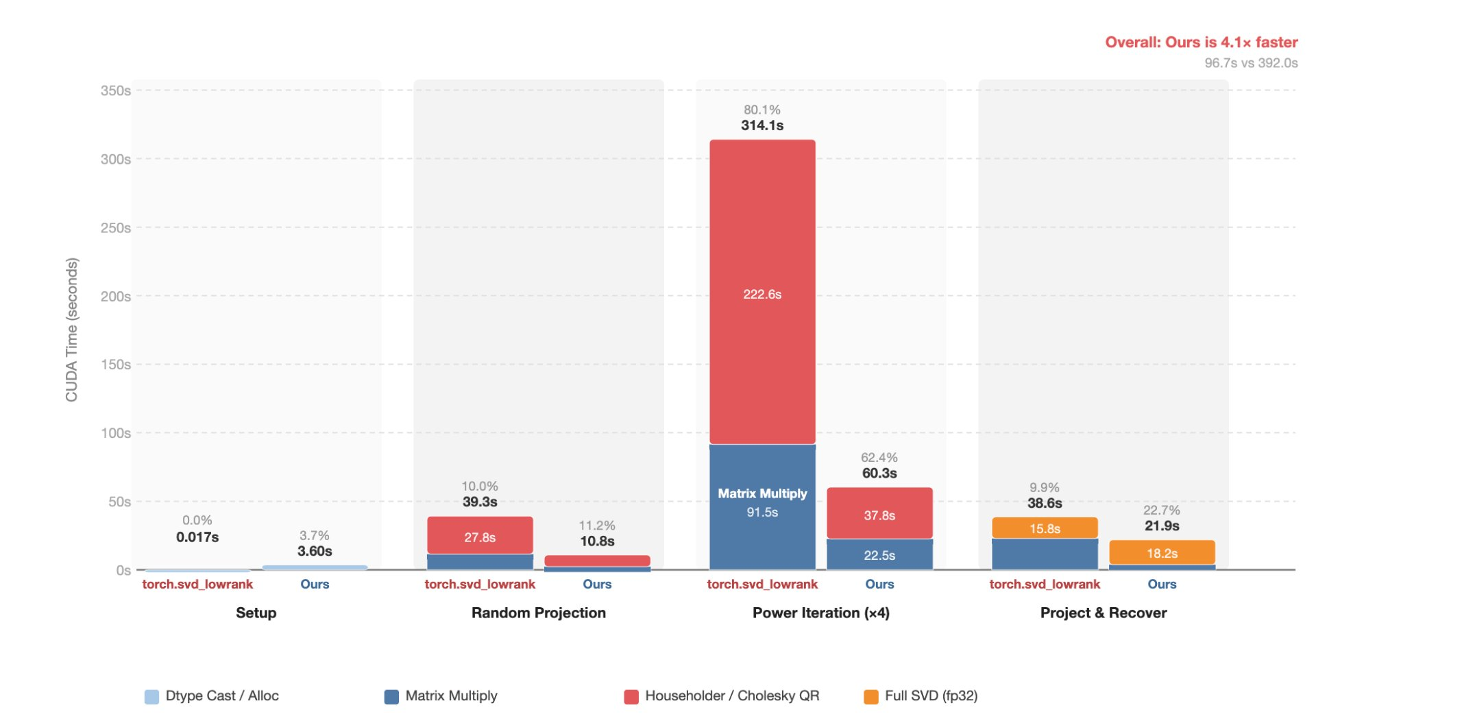
| Stage | fp32 · Householder QR | fp16 · Cholesky-QR (ours) | Speedup |
|---|---|---|---|
| 1. Setup (dtype cast / alloc) | 0.017 s (0.0%) | 3.60 s (3.7%) | — |
| 2. Random Projection | 39.3 s (10.0%) | 10.8 s (11.2%) | 3.6× |
| 3. Power Iteration (×4) | 314.1 s (80.1%) | 60.3 s (62.4%) | 5.2× |
| — Matrix Multiply | 91.5 s | 22.5 s | 4.1× |
| — Orthogonalization | 222.6 s | 37.8 s | 5.9× |
| 4. Project & Recover | 38.6 s (9.9%) | 21.9 s (22.7%) | 1.8× |
| Total | 392.0 s | 96.7 s | 4.1× |
Takeaways.
- Stage 1 adds 3.60 s of one-time dtype cast overhead, fully amortized by Stage 3 savings.
- Stage 3 is the primary bottleneck and primary gain. Power iteration drops from 314.1 s (80.1%) to 60.3 s (62.4%), a 5.2× speedup from two independent sources: matrix multiply improves 4.1× from Tensor Core utilization; orthogonalization improves 5.9× from Cholesky QR replacing Householder QR — a particularly large gain because Householder QR’s sequential panel structure is ill-suited to tall-and-skinny shapes with small $k+p$.
- Stage 4 shows a modest 1.8× gain from the 16-bit projection $B = Q^\top(A-M)$. Its share of total time grows from 9.9% to 22.7% — not because it became slower, but because Stage 3 shrank so dramatically.
6.4 Accuracy vs. Speed Trade-off
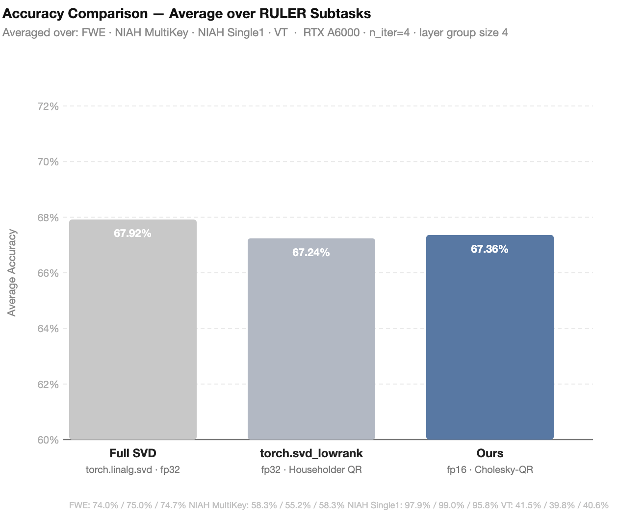
| Method | FWE | NIAH MultiKey | NIAH Single1 | VT | Average |
|---|---|---|---|---|---|
Full SVD (torch.linalg.svd) |
74.0% | 58.3% | 97.9% | 41.5% | 67.92% |
torch.svd_lowrank (baseline) |
75.0% | 55.2% | 99.0% | 39.8% | 67.24% |
| Ours (fp16 · Cholesky-QR) | 74.7% | 58.3% | 95.8% | 40.6% | 67.36% |
Takeaways.
- Averaged over all four RULER subtasks, our method (67.36%) matches the
torch.svd_lowrankbaseline (67.24%) within 0.12 percentage points — negligible accuracy cost for 4.1× lower SVD latency. - On two of four subtasks — NIAH MultiKey and VT — our method outperforms the baseline, reflecting that oversampling $p=4$ improves the quality of the random subspace estimate [1].
- A modest gap on NIAH Single1 (95.8% vs. 99.0%) likely reflects the slightly lower orthogonality of Cholesky QR for well-conditioned inputs [2] and minor 16-bit rounding in the power iteration.
7. Citing
@misc{abdelfattah2026svd_blog,
      title={Hardware efficient Randomized SVD},
      author={Zhihao Mo and Chi-Chih Chang and Mohamed Abdelfattah},
      year={2026},
      url={https://abdelfattah-lab.github.io/blog/svd_blog},
}
8. References
-
Halko, N., Martinsson, P. G., & Tropp, J. A. (2011). Finding structure with randomness: Probabilistic algorithms for constructing approximate matrix decompositions. SIAM Review, 53(2), 217–288. https://doi.org/10.1137/090771806
-
Fukaya, T., Nakatsukasa, Y., Yanagisawa, Y., & Yamamoto, Y. (2014). CholeskyQR2: A simple and communication-avoiding algorithm for computing a tall-skinny QR factorization on a large-scale parallel system. ScalA 2014, IEEE, pp. 31–38. https://doi.org/10.1109/ScalA.2014.11
-
Fukaya, T., Kannan, R., Nakatsukasa, Y., Yamamoto, Y., & Yanagisawa, Y. (2020). Shifted Cholesky QR for computing the QR factorization of ill-conditioned matrices. SIAM Journal on Scientific Computing, 42(1), A477–A503. https://doi.org/10.1137/18M1218212
-
Yamazaki, I., Tomov, S., & Dongarra, J. (2015). Mixed-precision Cholesky QR factorization and its case studies on multicore CPU with multiple GPUs. SIAM Journal on Scientific Computing, 37(3), C307–C330. https://doi.org/10.1137/14M0973773
-
Chang, C.-C., Lin, C.-Y., Akhauri, Y., Lin, W.-C., Wu, K.-C., Ceze, L., & Abdelfattah, M. S. (2025). xKV: Cross-layer SVD for KV-cache compression. arXiv:2503.18893.
-
Hsieh, C.-P., Sun, S., Kriman, S., Acharya, S., Rekesh, D., Jia, F., Zhang, Y., & Ginsburg, B. (2024). RULER: What’s the real context size of your long-context language models? arXiv:2404.06654.
-
Lee, F. What is singular value decomposition (SVD)? IBM Think. https://www.ibm.com/think/topics/singular-value-decomposition