

KV-Cache Refresh Methods for Long Generation


TL;DR
Refreshing a compressed KV cache every few decoding steps can improve long generation performance without significant overhead.
Introduction
Generating long, coherent, and high-quality text remains difficult for smaller open source language models. As sequences stretch into thousands of tokens, small decoding errors can compound. The model drifts from the prompt, repeats, or collapses into low information text. Practically, this isn’t just a language modeling issue, but it’s also a systems one. Prefill over the prompt is compute heavy but parallel, while decode is memory bandwidth bound and dominates wall-clock time, so simply using a bigger model everywhere isn’t viable at inference.
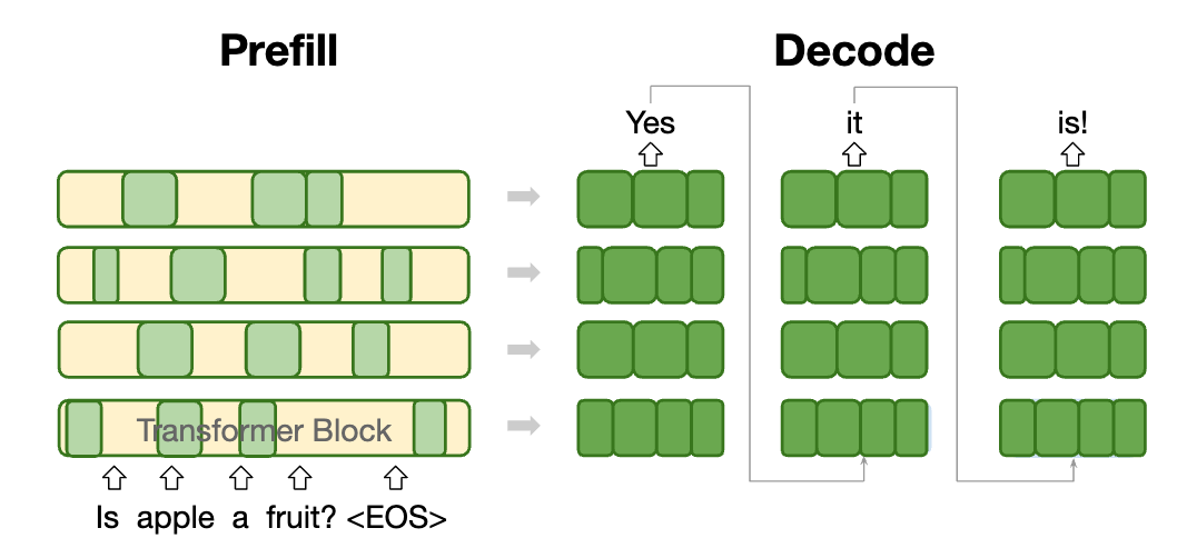
The OverFill architecture (Kim et al. 2025) exploits the prefill/decode split by running a large Teacher model only for the prefill to build a high-fidelity KV cache over the prompt, then hand that cache to a smaller Student model for the token by token decode. Prefill leverages parallelism to produce a strong initial state while decode runs much more quickly using the Student model. Below we formalize this prefill-decode setup (notation, algorithm).
In this blog, we perform dynamic KV cache refreshes to rebuild a high-fidelity KV cache during decoding. As KV cache refreshes do exert extra compute, we use them only when needed. This helps to realign the Student’s state to the Teacher’s state and to stabilize long generation for a small and controllable prefill tax.
We will analyze different methods of KV-cache refresh throughout this blog:
- Periodic refresh
- Entropy based refresh
- Speculative Refresh
- Monte Carlo Dropout (Future Work)
Background
Setup & Notation
- Prompt tokens: $x=(x_1,\ldots,x_L)$; generated tokens: $y_{1:N}$.
- Current sequence length at step $t$: $n_t \;=\; L + t$.
- Teacher model $T$ (higher quality) induces conditionals $p_T(\cdot\mid x,y_{<t})$.
- Student model $S$ (faster) induces $p_S(\cdot\mid x,y_{<t};\, C_{t-1})$.
-
Cache (per layer $\ell=1,\dots,L_{\text{layers}}$) stores keys/values up to time $t$:
\[K_{\ell,\le t}, V_{\ell,\le t}\;\in\;\mathbb{R}^{B \times H \times n_t \times d_h}, \qquad C_t \;\equiv\; \{K_{\ell,\le t}, V_{\ell,\le t}\}_{\ell=1}^{L_{\text{layers}}}.\] - NOTE: Passing KV across models is dimensionally valid if attention geometry and positional encoding match (same tokenizer/byte mapping, $H$, $d_h$, $L_{\text{layers}}$, RoPE/ALiBi params). Quality depends on model closeness; if geometry differs, rebuild the Student KV instead of reusing the Teacher’s.
The OverFill Algorithm (no refresh)
- Teacher prefill (build cache on prompt).
- Student decode (extend cache step-by-step). For $t=1..N$:
where the cache-update maps are
\[F_T:\ (C_{t-1}, y_t) \mapsto C_t^{(T)},\qquad F_S:\ (C_{t-1}, y_t) \mapsto C_t^{(S)}.\]Example code
# teacher prefill
kv = teacher(input_ids=ids_x, use_cache=True,
             past_key_values=DynamicCache()).past_key_values

# student decode
last = ids_x[:, -1:]
out = []
for _ in range(N):
    out_step = student(input_ids=last, past_key_values=kv, use_cache=True)
    logits = out_step.logits[:, -1, :]
    next_id = int(torch.argmax(logits, dim=-1))
    kv = out_step.past_key_values          # student appends new K/V
    out.append(next_id)
    last = torch.tensor([[next_id]], device=ids_x.device, dtype=ids_x.dtype)
Why Does OverFill Work?
(A) State alignment
Let $C_t^{(T)}$ and $C_t^{(S)}$ be the Teacher/Student cache trajectories, and define the error
\[E_t \;\triangleq\; C_t^{(S)} - C_t^{(T)}.\]Locally,
\[E_t \;\approx\; J_t\,E_{t-1} + \delta_t,\quad J_t \;=\; \left.\frac{\partial F_T}{\partial C}\right|_{C^{(T)}_{t-1}},\quad \delta_t \;=\; \left.(F_S - F_T)\right|_{C^{(T)}_{t-1}}.\]OverFill sets $E_0=0$ by starting from a Teacher-built $C_0$, reducing early compounding error vs. a pure-Student run.
(B) Variational lens
At step $t$, let $q_t(\cdot)=p_S(\cdot\mid x,y_{<t}; C_{t-1})$. Teacher-scored average log-prob satisfies
\[-\frac{1}{N}\sum_{t=1}^N \log p_T(y_t\mid\cdot) \;=\; \underbrace{\frac{1}{N}\sum_t \mathrm{KL}\!\big(p_T \,\|\, q_t\big)}_{\text{mismatch}} \;-\; \underbrace{\frac{1}{N}\sum_t H[p_T]}_{\text{fixed}},\]so lower PPL corresponds to smaller $\mathrm{KL}(p_T|q_t)$. OverFill shrinks this KL initially by providing a Teacher-consistent $C_0$.
Runtime
- Teacher prefill (once): $O(L)$ over the prompt (writes $C_0$).
- Student decode (per token): $O(1)$ w.r.t. $L$ using the cache.
- Throughput (TPS): essentially the Student’s decode TPS; OverFill overhead is the single Teacher prefill.
Overfill is advantageous for long prompts + short/medium outputs (by leveraging a strong initial state without incurring the large Teacher per-token cost). However, on very long outputs, Student drift accumulates, therefore motivating our KV-cache refresh.
KV Cache Refresh
During OverFill decode you maintain a KV cache $C_t$ as you append tokens. With a student $S$, the cache update map $F_S$ only approximates the teacher’s $F_T$, so errors can accumulate over decoding steps. A refresh discards the Student-evolved KV-cache, replacing it with a reconstructed KV-cache from the Teacher.
Formally, at step $t$ (with $n_t=L+t$):
\[\boxed{ \begin{aligned} \textbf{Decode (Student):}\;& y_t \sim p_S(\cdot \mid x, y_{<t};\, C_{t-1}),\quad C_t \leftarrow F_S(C_{t-1}, y_t). \\ \textbf{Refresh at } t\in R:\;& C_t \leftarrow \mathrm{Prefill}_T\!\big([x;\,y_{\le t}]\big). \end{aligned}}\]Incremental view: Keep a Teacher cache at the last refresh boundary $t’$. At refresh $t$, extend it only on the delta segment
\[\Delta_t \;\triangleq\; y_{t'+1:t}, \qquad |\Delta_t| = t - t',\]and condition the teacher on its cached prefix:
\[C_t^{(T)} \;\leftarrow\; \mathrm{Prefill}_T\!\big(\Delta_t;\ \text{past}=C_{t'}^{(T)}\big).\]Then realign the Student by splicing Teacher’s last $|\Delta_t|$ entries into the Student cache. Sliding window (optional). Limit correction to the last
\[k_t \;=\; \min\!\big(W,\ |\Delta_t|\big)\]positions per layer/head to cap cost and memory then splice only the last $k_t$.
Bayesian/Variational lens: Teacher log-prob on your outputs decomposes as>
\[-\frac{1}{N}\sum_{u=1}^N \log p_T(y_u\mid\cdot)\;=\;\frac{1}{N}\sum_u \mathrm{KL}\!\big(p_T\|q_u\big)\;-\;\frac{1}{N}\sum_u H[p_T].\]Refresh reduces $\mathrm{KL}(p_T|q_u)$ for subsequent tokens by re-anchoring the state.
KV compatibility: Passing KV across models is dimensionally valid if attention geometry and positional encoding match (same tokenizer/byte mapping, heads $H$, head size $d_h$, layers $L_{\text{layers}}$, and RoPE/ALiBi parameters). If geometry differs, do not reuse Teacher KV, but recompute the Student KV over the window from text.
Refresh Overhead
In general, the cost of adding refreshes is relatively inexpensive. Let refresh times be $t_1 < t_2 < \dots < t_R$ with $t_0 = 0$, and define
\[\Delta_r \;\triangleq \; y_{t_{r-1}+1:t_r},\quad m_r\;=\; |\Delta_r| \;=\; t_r - t_{r-1},\quad k_r \;=\; \min(W,\ m_r).\]With Student decode throughput $\mathrm{TPS}$ (tokens/s) over $N$ generated tokens,
\[\text{time} \;\approx\; \underbrace{\frac{N}{\mathrm{TPS}}}_{\text{Student decode}}\;+\; \underbrace{\sum_{r=1}^{R}\ \text{prefill}_{\mathrm{ms}}\big(k_r\big)}_{\text{Teacher spikes (incremental, windowed)}}.\]- Student decode TPS is unchanged by refresh (same kernels, same per-step work).
- Overhead is the Teacher prefill on the delta, capped by $W$ if using a sliding window.
Scheduling unification: Periodic refresh is just the same mechanism with stride $T$ (i.e., $m_r\approx T$); sliding-window sets $W<\infty$ to cap each spike. Speculative refresh uses fixed micro-bursts with $m_r=k$ every time, giving constant-cost spikes. Periodic with $W=T=k$ yields the same post-refresh KV as speculative for the last $k$ positions, so the differences are in granularity and cost shaping.
Periodic Refresh
A periodic refresh every $T$ tokens is the simplest approach. It rebuilds the Teacher cache incrementally on the last $T$ tokens, then splices the last $k=\min(W,T)$ positions into the Student cache.
@torch.no_grad()
def splice_last_k(student_kv, teacher_kv, k):
    # Replace only the last k time-steps per layer/head in the Student KV
    for layer in range(len(student_kv.key_cache)):
        sk, sv = student_kv.key_cache[layer], student_kv.value_cache[layer]
        tk, tv = teacher_kv.key_cache[layer], teacher_kv.value_cache[layer]
        if k > 0:
            sk[:, :, -k:, :] = tk[:, :, -k:, :]
            sv[:, :, -k:, :] = tv[:, :, -k:, :]
    return student_kv

@torch.no_grad()
def generate_with_refresh(teacher, student, tok, prompt, N=1000, T=64, W=None):
    # 1) Teacher builds C_0 on the prompt; mirror or rebuild for Student as needed
    from copy import deepcopy
    teacher_kv = teacher.prefill(prompt) # C_0^(T)
    student_kv = deepcopy(teacher_kv)  # or rebuild for Student if geometry differs

    out_ids = []
    t_last = 0

    for t in range(1, N + 1):
        # 2) Student decodes one token
        next_id, student_kv = student.step(out_ids[-1:], student_kv)
        out_ids.append(next_id)

        # 3) Periodic refresh every T tokens (incremental Teacher prefill on the delta)
        if t % T == 0:
            delta_ids = out_ids[t_last:t]            # Δ_r = y_{t_last+1 : t}
            teacher_kv = teacher.prefill(delta_ids, past_kv=teacher_kv)  # extend prefix
            k = t - t_last if W is None else min(W, t - t_last)
            student_kv = splice_last_k(student_kv, teacher_kv, k)
            t_last = t

    return tok.decode(out_ids)
Engineering notes.
- Use a unified cache object (e.g.,
DynamicCache) end-to-end; avoid tuple KV churn. - Keep RoPE base/scale (or ALiBi params) identical across Teacher & Student if you plan to splice; otherwise rebuild Student KV from text.
- Keep everything on-device; avoid unnecessary cache copies/boxing.
- Periodic $=$ stride $T$; sliding-window $=$ set $W$; speculative $=$ fix $m_r=k$ for constant-cost corrections.
Now, we test using 50 prompts for long form generation (1000+ tokens) using the ELI5 dataset, and evaluated using perplexity.
- Teacher:
meta-llama/Llama-3.2-3B-Instruct - Student:
friendshipkim/overfill-Llama-3.2-3B-Instruct-pruned-h0.45-i0.45-a0.0-d0.0 - Prompts: 50 long-form prompts
- Scoring: PPL, tail log-prob (last 50 toks under teacher), repetition\@3, character count, TTFT/TPS/total time
Baselines (no refresh)
| Policy | TTFT (s) | TPS (tok/s, decode) | Tokens (N) | Total (s, normalized) | End-to-end TPS (N/Total) | PPL ↓ | Repeat\@3 ↓ |
|---|---|---|---|---|---|---|---|
| Teacher | 0.040 | 28.2 | 1200 | 42.59 | 28.17 | 1.64 | 0.032 |
| OverFill | 0.191 | 28.5 | 1200 | 42.30 | 28.37 | 1.88 | 0.072 |
| Student | 0.041 | 29.4 | 1200 | 40.86 | 29.37 | 2.35 | 0.028 |
Takeaways.
- Quality: Teacher > OverFill > Student by PPL.
- Speed: Student is fastest but output collapses.
Periodic Refresh on OverFill
| Refresh $T$ | PPL ↓ | Latency Overhead |
|---|---|---|
| 0 (No Refresh) | 1.88 | 0% |
| 256 | 1.86 | +0.7% |
| 128 | 1.81 | +2.0% |
| 64 | 1.71 | +3.9% |
Gated Refresh
While effective, periodic refreshing is inefficient. It triggers a computationally expensive refresh even when the Student model is generating confidently. A more intelligent approach is to refresh on-demand, only when the model shows signs of uncertainty. In this section, we show how targeted refreshes can help, to find the optimal refresh times for more efficient implementations.
Entropy Gating
Use the Student next-token distribution $p_S(\cdot\mid x,y_{<t};C_{t-1})$ and refresh when its entropy exceeds a threshold $\tau$:
\[H_t^{(S)} \;=\; -\sum_{i} p_S(i\mid\cdot)\,\log_2 p_S(i\mid\cdot), \qquad \text{refresh if } H_t^{(S)} > \tau.\]This adds zero Teacher overhead until a refresh is actually triggered.
Optional (probe-KL every $M$ steps). If you want a teacher-anchored signal without paying per-token cost, probe every $M$ steps:
- compute $p_T(\cdot\mid\cdot)$ only at probe steps,
- measure $\mathrm{KL}!\big(p_T|p_S\big)$, and refresh if it exceeds $\kappa$. This bounds Teacher calls to $\lfloor N/M\rfloor$ probes.
Budgeting. Choose $\tau$ (or $\kappa$) to target ~2–3 refreshes per 1k tokens (or any budget you want). You can estimate $\tau$ from the 95th–97th percentile of $H_t^{(S)}$ on a small calibration set.
Results ($N=1200$ tokens)
| Entropy $\tau$ (bits) | Avg #Refresh | PPL ↓ | Total (s) | TPS |
|---|---|---|---|---|
| 5.5 | 2.5 | 1.70 | 35.42 | 28.6 |
| 6.0 | 2.0 | 2.27 | 35.34 | 28.3 |
| 6.5 | 1.5 | 2.19 | 35.97 | 27.8 |
We see targeted refreshes achieve as low perplexity as the T=64 refresh, but is faster now, since we only refresh when needed!
Speculative Refresh
Full or sliding-window refreshes rebuild a long span of cache. Speculative Refresh keeps Teacher work constant by operating in short bursts.
Algorithm (burst size $k$):
- Student speculation. Generate $k$ tokens, updating the Student cache:
- Teacher correction (incremental). Extend the Teacher cache only on the new segment $\Delta_{t+k} = y_{t+1:t+k}$ using the Teacher’s prefix at $t$:
- Cache splicing (last $k$). Replace only the last $k$ time-steps per layer/head in the Student cache with the Teacher’s entries:
Repeat. This keeps the Student trajectory close to the Teacher while the Teacher’s workload is constant (size $k$ per refresh).
Relation to periodic. Periodic with stride $T=k$ and window $W=k$ produces the same post-refresh KV on the last $k$ tokens. The difference is cost shaping and granularity: speculative ensures small, regular, GPU-friendly spikes; periodic cost grows with the time since the last refresh unless windowed.
Results
The key advantage is that the teacher’s workload is constant and small (always processing $k$ tokens), unlike a full refresh where the prefill cost grows with the sequence length.
| Refresh Method | Refresh Cost | Latency Overhead | PPL |
|---|---|---|---|
Periodic (T=64) |
Grows with sequence length | ~3.9% | 1.71 |
Speculative (k=8) |
Constant (prefill over 8 tokens) | ~1.9% | 1.77 |
NOTE: Only preliminary results over 1 run of $k$.
Future Work (Monte Carlo Dropout)
The entropy-gated approach is an effective heuristic, but it doesn’t distinguish between two fundamentally different types of uncertainty (Aleatoric, Epistemic).
A more principled approach is to isolate epistemic uncertainty directly. We can achieve this by treating the student decoder as an approximation of a Bayesian Neural Network (BNN) using Monte Carlo (MC) Dropout.
As shown by Gal & Ghahramani (2016), a standard neural network trained with dropout can be interpreted as an approximation to a deep Gaussian process. By keeping dropout active during inference, we can sample from the model’s approximate posterior distribution. Each forward pass with a different dropout mask yields a different prediction; the variance across these predictions is a direct measure of epistemic uncertainty.
Mathematical Formulation
At each decoding step $t$, instead of a single forward pass, we perform $N$ stochastic forward passes with the student model $\theta’$:
\[\boldsymbol{z}_i = f_{\theta', \boldsymbol{m}_i}(y_{t-1}, K_{t-1}) \quad \text{for } i=1..N\]where $m_i \sim \text{Bernoulli}(1-p)$ is a random dropout mask. This gives us a set of logit vectors $z_1, \ldots, z_N$. We then quantify epistemic uncertainty by calculating the total variance, approximated by the mean of the variances across each logit dimension:
\[U(t) = \frac{1}{D_{vocab}} \sum_{j=1}^{D_{vocab}} \text{Var}(\{\boldsymbol{z}_{i,j}\}_{i=1}^N)\]A high $U(t)$ signifies that the student’s predictions are unstable—a clear signal of high epistemic uncertainty.
Simulation & Expected Results
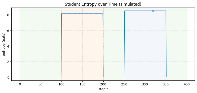
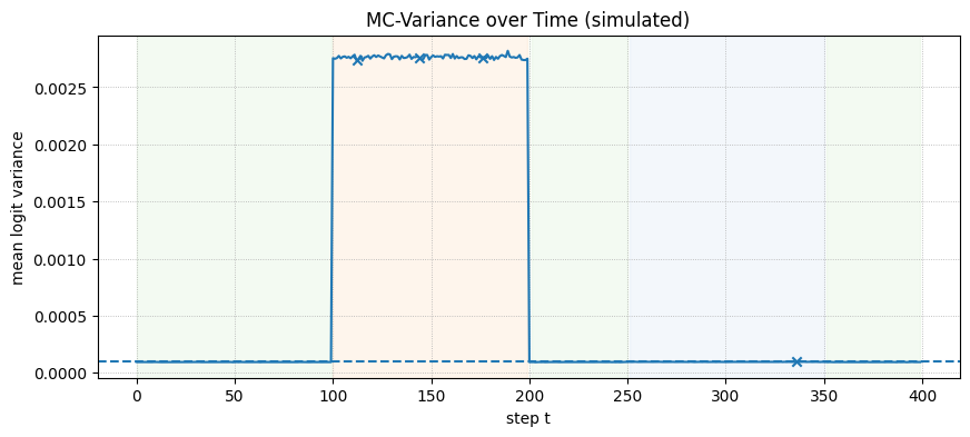
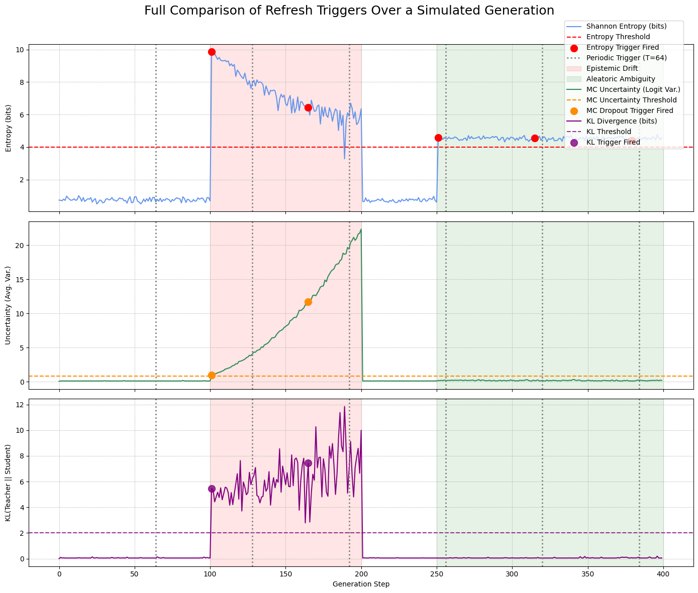
While implementing true MC Dropout requires a model trained with dropout layers, we can simulate its behavior over a 400-step generation that includes phases of confidence, epistemic drift, and aleatoric ambiguity.
- Confident Start (Steps 0-100): The model is certain, so entropy and variance are low.
- Epistemic Drift (Steps 100-200): The model gets confused. Internal states become unstable, causing high variance between stochastic forward passes. This also flattens the output distribution, leading to high entropy.
- Post-Refresh Confidence (Steps 201-250): A hypothetical refresh resets the model to a confident state.
- Aleatoric Ambiguity (Steps 251-350): The model encounters a genuinely ambiguous next step (e.g., “The prize could be a car or a…”). It is confidently uncertain, so the output distribution is flat (high entropy), but the variance between stochastic passes is low.
The plot shows that the MC Uncertainty trigger would correctly remains silent during the aleatoric (ambiguous) phase, while the entropy trigger incorrectly fires. The MC dropout approach can be an efficient alternative to try out.
Phase summary
| phase | steps | mean_entropy | mean_mcvar | frac_entropy_fire | frac_mcvar_fire |
|---|---|---|---|---|---|
| alea | 100 | 8.5172 | 0.0001 | 0.01 | 0.01 |
| conf | 150 | 0.0096 | 0.0001 | 0.00 | 0.00 |
| drift | 100 | 8.1466 | 0.0028 | 0.00 | 0.03 |
| post | 50 | 0.0096 | 0.0001 | 0.00 | 0.00 |
Thresholds: tau_entropy=8.5172 nats, tau_mcvar=0.000096 Entropy fires at: [320] MC-variance fires at: [112, 144, 176, 336]
Conclusion
Refreshing the KV cache makes small decoders behave more like big ones on long generations. Starting from OverFill, a simple periodic policy already closes most of the quality gap (e.g., T=64 improves PPL from ~1.88 → ~1.71 at only ~4% extra latency). An entropy-gated policy reaches the same quality with fewer, better-timed refreshes, and speculative refresh keeps Teacher work constant (e.g., k=8–16) so spikes stay tiny (~2% overhead) while maintaining near-periodic quality. Future work can explore uncertainty-aware refresh triggers such as MC Dropout to estimate epistemic uncertainty and trigger refreshes only when model belief is unstable, so we can match or exceed entropy-gated quality under the same refresh budget.
Citing
@misc{abdelfattah2025_overfill_blog,
      title={KV-Cache Refresh Methods for Long Generation},
      author={Yahya Emara and Woojeong Kim and Mohamed Abdelfattah},
      year={2025},
      url={https://abdelfattah-lab.github.io/blog/overfill_refresh},
}